Part I - Differential Equations

Classifying Ordinary Differential Equations (ODEs)

Linear Homogeneous

A linear ODE is defined using:

If the term contains one and only one factor which is a dependent variable or the derivative of a dependent variable then the term is linear in the dependent variable.

Furthermore, a linear homogeneous ODE is defined using:

If each term of the ODE is linear in the dependent variable or zero, then the ODE is linear homogeneous.

Example: \[\frac{d^2x}{dt^2}+a(t)\frac{dx}{dt}+x(t)=0\]

Linear Inhomogenous

Definition:

If you can write each equation in a form where the left hand side is a linear homogeneous ODE, and the right hand side is non zero and does not contain any dependent variables or their derivatives, then the ODE is linear inhomogeneous.

Example: \[\frac{d^2x}{dt^2}+a(t)\frac{dx}{dt}+x(t)=b(t)+\sin(t)\]

Non linear

All other ODEs are non linear

Example: \[\left(\frac{dx}{dt}\right)^2+a(t)\frac{dx}{dt}+x(t)=0\] NOTE: These classifications also apply to partial differential equations, as the only difference is the quantity of independent variables, not dependent. Also, \(\nabla\) is a linear operator, such that it may be in linear ODEs.

Properties of ODEs

Linear Homogeneous ODEs

Linear homogeneous ODEs have two important properties.

• Given a solution \(f(t)\) to a linear homogeneous ODE, \(\lambda f(t)\) is also a solution, where \(\lambda\) is an arbitrary constant.
• Given two solutions \(f(t)\) and \(g(t)\) to a lin. hom. ODE, \(h=f+g\) is also a solution.

Linear Inhomogeneous ODEs

The homogeneous part of a linear inhomogeneous equation is obtained by setting all the terms not containing a dependent variable to zero.

• Given a solution \(f(t)\) to a linear inhomogeneous ODE and \(g(t)\) is a solution to the homogeneous part, then \(h(t)=f(t)+g(t)\) is a solution to the linear inhomogeneous equation.

Separation of Variables

Lets learn this by example. Take the wave equation in \((t,x)\). \[\frac{\partial^2\psi}{\partial t^2}-\frac{\partial^2\psi}{\partial x^2}=0\] Now we propose the following ansatz: \[\psi(t,x)=\alpha(t)\beta(x)\] We can derive that \[\frac{d^2\alpha(t)}{dt^2}\frac{1}{\alpha(t)}=\frac{d^2\beta(x)}{dx^2}\frac{1}{\beta(x)}\] This is the crucial part. We can observe that the LHS depends only on \(t\), while the RHS depends only on \(x\). Therefore they must equal each other \(\forall (x,t)\), hence they must equal a constant. \[\implies\frac{d^2\alpha}{dt^2}\frac{1}{\alpha}=\frac{d^2\beta}{dx^2}\frac{1}{\beta}=C,\] where \(C\) is called the constant of separation.

We can choose the form of the constant of separation, and here we should choose \(C=-\omega^2\). Thus we find: \[\frac{d^2\alpha}{dt^2}\frac{1}{\alpha}=-\omega^2\qquad\qquad\frac{d^2\beta}{dx^2}\frac{1}{\beta}=-\omega^2\] Thus: \[\begin{align} \alpha=A\cos(\omega t)+B\sin(\omega t)\\\beta=C\cos(\omega x)+D\sin(\omega x) \end{align}\] ...and since \(\psi(t,x)=\alpha(t)\beta(x)\): \[\psi(t,x)=\left[A\cos(\omega t)+B\sin(\omega t)\right]\left[C\cos(\omega x)+D\sin(\omega x)\right]\] Note that this is equivalent to: \[\begin{align} &\psi(t,x)=A\cos(\omega t)\cos(\omega x)+B\cos(\omega t)D\sin(\omega x)\\ &+C\sin(\omega t)\cos(\omega x) + D\sin(\omega t)\sin(\omega x) \end{align}\] where the constants are redefined. These are the general solutions to the equation.

Wave Equation: Initial & Boundary Conditions

• The permissible frequencies \(\omega_n\) are determined by the boundary conditions.
• We assume we have an elastic string of length \(L\), that is fixed at both ends. Thus we impose: \[\psi(t, 0)=0,\qquad\qquad\psi(t,L)=0\]
• We can also impose arbitrary initial conditions: \[\psi(0, x)=\psi_0(x)\qquad\qquad\left.\frac{\partial\psi}{\partial t}\right|_{t=0}=\psi_1(x)\]

We use these with the general solution to find that \[\begin{align} &A=0,\qquad C=0,\qquad\sin(\omega L)=0\\ &\implies\omega_n=\frac{\pi n}{L},\;\;n\in\mathbb{Z}^+ \end{align}\] Since the wave equation is homogeneous linear we can add arbitrary solutions with different \(\omega\). Thus the solution for the specified boundary conditions is given by: \[\psi(t,x)=\sum^\infty_{n-1}\left(B_n\cos\left(\frac{\pi n}{L}t\right)\sin\left(\frac{\pi n}{L}x\right)+D_n\sin\left(\frac{\pi n}{L}t\right)\sin\left(\frac{\pi n}{L}x\right)\right)\] Now we can apply the initial conditions to further simplify the solution. We set \(t=0\) and also differentiate the result and set \(t=0\) to find: \[\psi_0(x)=\sum^\infty_{n=1}B_n\sin\left(\frac{n\pi}{L}x\right) \] \[\psi_1(x)=\sum^\infty_{n=1}\frac{n\pi}{L}D_n\sin\left(\frac{n\pi}{L}x\right) \] We now use the fact that \[\frac{2}{L}\int^L_0\sin\left(\frac{n\pi}{L}x\right)\sin\left(\frac{m\pi}{L}x\right)\;dx=\left\{ \begin{align} &1\;\;\;\;\textrm{if}\;n=m\\ &0\;\;\;\;\textrm{if}\;n\neq m \end{align}\right.\] to rearrange \(\psi_0\) to find: \[B_m=\frac{2}{L}\int^L_0\sin\left(\frac{m\pi}{L}x\right)\psi_0(x)\;dx \] We can do the same technique with \(\psi_1\) to get: \[D_m=\frac{2}{m\pi}\int^L_0\sin\left(\frac{m\pi}{L}x\right)\psi_1(x)\;dx \] So we can get the general solution: \[\psi(t,x)=\sum_{n=1}^\infty B_n\cos\left(\frac{n\pi}{L}t\right)\sin\left(\frac{n\pi}{L}x\right)+\sum_{n=1}^\infty D_n\sin\left(\frac{n\pi}{L}t\right)\sin\left(\frac{n\pi}{L}x\right)\] where \[\begin{align} &B_n=\frac{2}{L}\int^L_0\sin\left(\frac{n\pi}{L}x\right)\psi_0(x)\;dx\\ &D_n=\frac{2}{n\pi}\int^L_0\sin\left(\frac{n\pi}{L}x\right)\psi_1(x)\;dx \end{align}\]

Spherical Harmonics

Laplace Operator in Spherical Coordinates

Recall this from PHYS115: \[\Delta\psi=\frac{1}{r^2}\frac{\partial}{\partial r}\left(r^2\frac{\partial\psi}{\partial r}\right)+\frac{1}{r^2\sin\theta}\frac{\partial}{\partial\theta}\left(\sin\theta\frac{\partial\psi}{\partial\theta}\right)+\frac{1}{r^2\sin^2\theta}\frac{\partial^2\psi}{\partial\phi^2}\] We can rewrite this as \[\Delta\psi=\frac{1}{r^2}\frac{\partial}{\partial r}\left(r^2\frac{\partial\psi}{\partial r}\right)+\frac{1}{r^2}\Delta_{\textrm{sph}}\psi\] where \[\Delta_{\textrm{sph}}\psi=\frac{1}{\sin\theta}\frac{\partial}{\partial\theta}\left(\sin\theta\frac{\partial\psi}{\partial\theta}\right)+\frac{1}{\sin^2\theta}\frac{\partial^2\psi}{\partial\phi^2}\] is the Laplace operator on the sphere.

Spherical Wave Equation

First we shall solve the spherical wave equation \[\frac{\partial^2\psi}{\partial t^2}-\Delta_{\textrm{sph}}\psi=0\qquad\textrm{for}\qquad\psi=\psi(t,\theta,\phi)\]

• We may think of a rubber ball, with air inside. Let \(\psi\) be the radial displacement of the ball from the rest spherical position.
• For small displacements and a short period of time, the spherical wave equation is a reasonable model for the motion of the surface of the ball.
• However it is linear, so is a bad approximation for large displacements, and there is no damping term so the motion will continue for ever.
• Particular solutions are called spherical harmonics.

We shall separate \(t\), first then \((\theta,\phi)\). Thus let \(\psi(t,\theta,\phi)=\alpha(t)+\Upsilon(\theta,\phi)\) \[\implies\frac{d^2\alpha}{dt^2}+\omega^2\alpha=0\qquad\&\qquad\Delta_\textrm{sph}\Upsilon+\omega^2\Upsilon=0\] hence, the \(\alpha\) equation is solved for fixed frequency by setting \[\alpha(t)=A_\omega\cos(\omega t)+B_\omega\sin(\omega t)\] For the \(\Upsilon\) equation, we shall set \(\omega^2=n(n+1)\) where \(n\) is an integer. (This is dictated later). \[\frac{1}{\sin\theta}\frac{\partial}{\partial\theta}\left(\sin\theta\frac{\partial\Upsilon}{\partial\theta}\right)+\frac{1}{\sin^2\theta}\frac{\partial^2\Upsilon}{\partial\phi^2}+n(n+1)\Upsilon=0\] We shall again use a separation of variables, and set \(\Upsilon(\theta,\phi)=W(\theta)V(\phi)\) \[\implies\frac{1}{\sin\theta}\frac{d}{d\theta}\left(\sin\theta\frac{dW}{d\theta}\right)+\left(n(n+1)-\frac{m^2}{\sin^2\theta}\right)W=0\] and \[\frac{d^2V}{d\phi^2}+m^2V=0\] The latter is clearly another simple harmonic oscillator, however the boundary conditions are now periodic since \(\phi\) is an angle. Thus \[V(\phi)=V(\phi+2\pi)\] The previous sine and cosine solutions do not work in this case, so we adopt the exponential form \[V(\phi)=Ae^{im\phi}+Be^{-im\phi}\]

• For this to be periodic, we require \(m\in\mathbb{z}\).
• For real solutions of the wave equation we must take the real part \(\psi(t,\theta,\phi)=\textrm{Re}(\alpha(t)W(\theta)V(\phi))\)

As for the former equation we need to convert to the associated Legendre equation.

• We substitute \(z=\cos\theta\) and set \[P(z)=P(\cos\theta)=W(\theta)\]
• We differentiate both sides by \(\theta\) to get \[-\sin\theta\frac{dP}{dz}(\cos\theta)=\frac{dW}{d\theta}\] Thus \[-\sin^2\theta\frac{dP}{dz}(\cos\theta)=\sin\theta\frac{dW}{d\theta}\]
• We repeat this step to get \[\sin\theta\frac{d}{dz}\left(\sin^2\theta\frac{dP}{dz}(\cos\theta)\right)=\frac{d}{d\theta}\left(\sin\theta\frac{dW}{d\theta}\right)\] Hence \[\frac{d}{dz}\left(\sin^2\theta\frac{dP}{dz}(\cos\theta)\right)=\frac{1}{\sin\theta}\frac{d}{d\theta}\left(\sin\theta\frac{dW}{d\theta}\right)\]
• We substitute this into the equation to find \[\frac{d}{dz}\left(\sin^2\theta\frac{dP}{dz}(\cos\theta)\right)+\left(n(n+1)-\frac{m^2}{\sin^2\theta}\right)P=0\]
• Since \(z=\cos\theta,\;\;\sin^2\theta=1-\cos^2\theta=1-z^2\), we get \[\frac{d}{dz}\left((1-z^2)\frac{dP}{dz}\right)+\left(n(n+1)-\frac{m^2}{1-z^2}\right)P=0\]

This is the Associated Legendre Equation. Since \(P\) clearly depends on \(n\) and \(m\) as well as \(z\), we write \(P_n^m(z)\). Thus we have the A.L.E. \[\frac{d}{dz}\left((1-z^2)\frac{dP^m_n}{dz}\right)+\left(n(n+1)-\frac{m^2}{1-z^2}\right)P_n^m=0\] This is a second order linear ODE. Therefore there are two solutions.

• If \(n\in\mathbb{N}\) and \(m=-n,-n+1,\dots,n-1,n\) there is one bounded solution, i.e. does not go to infinity for any \(z=[-1,+1]\). This is the associated Legendre polynomial \[P^m_n(z)=\frac{1}{2^nn!}(1-z^2)^{m/2}\frac{d^{n+m}}{dz^{n+m}}(z^2-1)^n.\]
• If \(n,m\) are not in this range, there is no bounded solution.
• Observe that if \(m\) is odd, then \(P^m_n\) is not a polynomial, however the name has stuck.

Up to \(\pm 1\) the spherical harmonics are given by \[Y^m_n(\theta,\phi)=\left(\frac{2n+1}{4\pi}\frac{(n-m)!}{(n+m)!}\right)^{1/2}e^{im\phi}P_n^m(\cos\theta)\] where \(P^m_n\) is as above. The solution to the wave equation for \(\psi=\psi(t,\theta,\phi)\) is \[\psi=\sum^\infty_{n=0}\sum^n_{m=-n}\left(A_{mn}\cos\left(\sqrt{n(n+1)t}\right)+B_{nm}\sin\left(\sqrt{n(n+1)t}\right)\right)Y^m_n(\theta,\phi)\]

Laplace's Equation

Laplace's Equation for \(\psi(r,\theta,\phi)\) is \[\Delta\psi=0\] We can use the definition of the Laplacian in spherical coordinates as given above and use \[\Delta_\textrm{sph}Y^m_n=-n(n+1)Y^m_n\] with the separation of variables \(\psi(r,\theta,\phi)=R(r)\Upsilon(\theta,\phi)\) to find the radial equation \[\frac{d}{dr}\left(r^2\frac{dR}{dr}\right)=n(n+1)R\] We now use the ansatz \(R(r)=r^\alpha\). \[\implies\alpha(\alpha+1)=n(n+1)\] hence \(\alpha=n\) and \(\alpha=-n-1\). Therefore the solution to Laplace's equation is \[\psi(r,\theta,\phi)=\sum^\infty_{n=0}\sum^n_{m=-n}B_{nm}r^{-n-q}Y^m_n(\theta,\phi)\]

Bessel Functions

Wave Equation on a Disk

The wave equation on the disc for the scalar \(\psi=\psi(t,\rho,\theta)\) is given by \[\frac{\partial^2\psi}{\partial t^2}-\Delta_\textrm{disc}\psi=0\] where the Laplace operator in plane polar coordinates is \[\Delta_\textrm{disc}\psi=\frac{1}{\rho}\frac{\partial}{\partial\rho}\left(\rho\frac{\partial\psi}{\partial\rho}\right)+\frac{1}{\rho^2}\frac{\partial^2\psi}{\partial\theta^2}\] Again, we use separation of variables \(\psi=\alpha(t)\mathcal{J}(\rho,\theta)\) to give \[\frac{d^2\alpha}{dt^2}+\omega^2\alpha=0\qquad\&\qquad\Delta_\textrm{disc}\mathcal{J}(\rho,\theta)+\omega^2\mathcal{J}=0\] We are then left with the equation using the disk Laplace operator \[\Delta_\textrm{disc}\mathcal{J}=\frac{1}{\rho}\frac{\partial}{\partial\rho}\left(\rho\frac{\partial\mathcal{J}}{\partial\rho}\right)+\frac{1}{\rho^2}\frac{\partial^2\mathcal{J}}{\partial\theta^2}=-\omega^2\mathcal{J}\] where \(\mathcal{J}=\mathcal{J}(\rho,\theta)\). This we can solve by separation of variables, setting \(\mathcal{J}=P(\rho)W(\theta)\). Using \(-m^2\) as the constant of separation gives \[\begin{align} &\frac{d^2W}{d\theta^2}+m^2W=0\\ &\rho\frac{d}{d\rho}\left(\rho\frac{dP}{d\rho}\right)+(\omega^2\rho^2-m^2)P=0 \end{align}\] The solution to the first equation is \[W=A\cos(m\theta)+B\sin(m\theta)\] Since \(\theta\) is an angle, as before, \(m\in\mathbb{z}\). There is also a zero mode, when \(m=0\), so that \(W''=0\), which is solved by \[W=W_0=A_0+B_0\theta\] but from periodicity, \(B_0=0\).

We solve the second equation by transforming \(P(\rho)\) into Bessel's equations, by setting \(\rho=x/\omega\) and \(P(\rho)=y(x)\). Thus \[\frac{d}{d\rho}=\omega\frac{d}{dx}\] Giving \[x\frac{d}{dx}\left(x\frac{dy}{dx}\right)+(x^2-m^2)y=0\] where \(m\in\mathbb{z}\). This is Bessel's equation of order \(m\).

These are solved by Bessel functions. Since this equation is second order, we know that there are two solutions, \[y(x)=J_m(x)\qquad y(x)=Y_m(x)\] respectively called Bessel functions of the first and second kind. In the limit \(x\to0\), \(J_m\) is a finite quantity, whereas \(Y_m\to-\infty\).

Since \(x=0\) corresponds to \(\rho=0\), we require the coefficient of \(Y_m\) be zero. Thus \(y(x)=AJ_m(x)\).

After long calculation, it can be shown that \[J_m(x)=\sum^\infty_{s=0}\frac{(-1)^sx^{m+2s}}{2^{m+2s}s!(m+s)!}\] Plotting the first six Bessel functions (of the first kind) gives: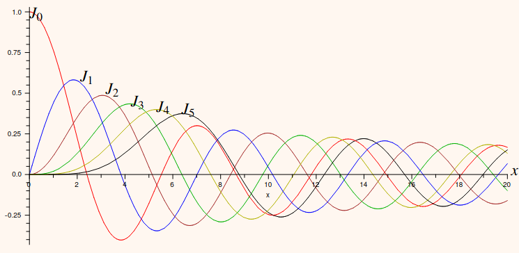

Hence, for a fixed frequency \(\omega\), our solutions to \(\Delta_\textrm{disk}\mathcal{J}=-\omega^2\mathcal{J}\) are: \[\begin{array}{c} \mathcal{J}(\rho,\theta)=\cos(m\theta)J_m(\omega\rho)\\ \mathcal{J}(\rho,\theta)=\sin(m\theta)J_m(\omega\rho)\\ \implies\mathcal{J}=A\cos(m\theta)J_m(\omega\rho)+B\sin(m\theta)J_m(\omega\rho)\end{array}\] Solving the \(\alpha\) is trivial, it its a simple harmonic oscillator again, where the steps to solve are detailed above. We get \[\alpha(t)=C\cos(\omega t)+D\sin(\omega t)\] Thus, the solutions to the wave equation \(\frac{\partial^2\psi}{\partial t^2}+\Delta_\textrm{disk}\psi=0\) are \[\begin{array}{l} \psi(t,\rho,\theta)=\alpha(t)\mathcal{J}(\rho,\theta)\\ \implies\psi=[A\cos(m\theta)J_m(\omega\rho)+B\sin(m\theta)J_m(\omega\rho)][C\cos(\omega t)+D\sin(\omega t)] \end{array}\]

Boundary Conditions

Now we must involve boundary conditions to find the possible values of \(\omega\).

• Let us consider a disk of radius \(R\). We impose the boundary condition that \(\psi(t,R,\theta)=0\), that is \(\rho=R\).
• Thus, for each integer \(m\geq0\), we have \(J_m(\omega R)=0\)
• Enumerate all of the roots of \(J_m\). That is let \(\chi^s_m\) be the \(s\)'th root of \(J_m\) so that \(J_m(\chi^s_m)=0\)
• Since for \(m\gt 0\), \(J_m(0)=0\), we set \(\chi^0_m=0\).
• We find \(\omega=\frac{\chi^s_m}{R}\)

Thus \[\psi=\sum^\infty_{m=0}\sum^\infty_{d=0}\left(\left[A_{ms}\cos(m\theta)J_m\left(\frac{\chi^s_m}{R}\rho\right)+B_{ms}\sin(m\theta)J_m\left(\frac{\chi^s_m}{R}\rho\right)\right]\left[C_{ms}\cos\left(\frac{\chi^s_m}{R} t\right)+D_{ms}\sin\left(\frac{\chi^s_m}{R} t\right)\right]\right)\] where \(A_{ms},\;B_{ms},\;C_{ms},\;D_{ms}\) are determined by the initial conditions.

Circular Wave Guides

We can promote \(\psi(t,\rho,\theta)\to\psi(t,\rho,\theta,z)\) so that \[\frac{\partial^2\psi}{\partial t^2}-\Delta_\textrm{disk}\psi\quad\to\quad\frac{\partial^2\psi}{\partial t^2}-\Delta_\textrm{disk}\psi-\frac{\partial^2\psi}{\partial z^2}=0\] we can use SOV again with \(\psi=\alpha(t)\beta(\rho,\theta)\gamma(z)\), to show that \[\begin{array} &\frac{d^2\alpha}{dt^2}=-\omega^2\alpha\quad &\Delta_\textrm{disk}\beta=-k^2\beta\quad &\frac{d^2\gamma}{dz^2}=\varepsilon\mu^2\gamma \end{array}\] with \(k=\chi^s_m/R\), \(\varepsilon=\pm1\) and \(\omega^2=k^2-\varepsilon\mu^2\). The sign of \(\varepsilon\) determine if the waves are propagating or non propagating.

• \(\varepsilon=1\) the waves are non propagating.
• \(\varepsilon=-1\) the waves are non propagating.

Part II - Linear Algebra

We will write \(A\in M_{m\times n}(\mathbb{R})\) to mean \(A\) is an \(m\times n\) real matrix with \(m\) rows and \(n\) columns, and \(A\in M_{m\times n}(\mathbb{C})\) to mean the corresponding complex matrix.

• A matrix with all zero entries is called the zero matrix. It may be written \(0_{m\times n}\).
• The \(n\)-vector with all zero entries is called the zero vector and may be written \(\mathbf{0}_n\). If \(n\) is unambiguous, we skip the index.
• A matrix where \(m=n\) is called a square matrix.
• A square matrix where the main diagonal is populated with 1's, and 0's everywhere else is called the identity matrix. We use the symbol \(I\) for the identity matrix, and can add an index should we wish.

Common Matrix Operations

Two matrices \(A\) and \(B\) may be added to form a matrix \(C\) ONLY IF \(m_A=m_B\) and \(n_A=n_B\). \[C=A+B\] To perform this, simply add the \((i,j)\)th element of the first matrix to the \((i,j)\)th element of the second matrix to also get the \((i,j)\)th element of the third matrix.

A matrix may be multiplied by a scalar by simply multiplying each element by the scalar. \[\lambda\begin{pmatrix}a&b\\d&e\end{pmatrix}=\begin{pmatrix}\lambda a&\lambda b\\\lambda d&\lambda e\end{pmatrix}\] Matrix multiplication is more complicated. For \(A\in M_{m,n},\;B\in M_{r,s}\) we require that \(n=r\), and the resulting matrix will be \(AB\in M_{m,s}\) .

A trick to remember this is that for \(M_{m,n},\;M_{r,s}\) the inside indices must be the same, and the result will be of dimensions of the outside indices. \[\begin{pmatrix} a&b&c\\d&e&f \end{pmatrix}\begin{pmatrix} g&h\\i&j\\k&l \end{pmatrix}=\begin{pmatrix} A&B\\C&D \end{pmatrix}\] where \[\begin{align} &A=ag+bi+ck\\ &B=ah+bj+cl\\ &C=dg+ei+fk\\ &D=dh+ej+fl \end{align}\] We have multiplied two matrices by taking the dot product of the \(m\)th row of the first matrix by the \(n\)'th column of the second matrix, to give the corresponding \((m,n)\)th entry of the result.

Index notation for matrices and vectors.

Some set notation: \(A\in\mathbb{C}\), A is in the set of complex numbers. \(\{1,2,3\}\subset\mathbb{R}\), \(\{1,2,3\}\) is a subset of the real numbers. To notate a real \(n\)-vector, we write \(A\in\mathbb{R}^n\).

Given a matrix \(A\), we represent the \((i,j)\)'th entry by the symbol \(A_{ij}\).

• The advantage of this notation is that it can be used for matrix and vector expressions.
• Thus for matrices \(A\) and \(B\) and a scalar \(\lambda\), then the symbol \((A+\lambda B)_{ij}\) means the entry \(C_{ij}\) of the matrix \(C=A+\lambda B\)

So for matrix multiplication we can find that \[(AB)_{ij}=\sum^n_{k=1}A_{ik}B_{kj}\] where \(A\in M_{a,n},\;B\in M_{n, b}\). Where \(a,b\) are arbitrary constants.

Kronecker Delta

Remember the identity matrix is \[I_n=\pmatrix{ 1&0&\ldots&0\\ 0&1&\ddots&\vdots\\ \vdots&\ddots&1&0\\ 0&\ldots&0&1 }\in M_{n\times n}(\mathbb{R})\] In components, \[(I_n)_{ij}=\left\{\begin{align}&1\quad \textrm{if}\;i=j\\&0\quad\textrm{if}\;i\neq j\end{align}\right.\quad =\delta_{ij}\] This is very useful in index notation proofs.

Rules for addition and (scalar) multiplication

For addition and scalar multiplication, the algebraic rules are nothing special. There is associativity, addition of zero, distributivity and commutativity. Its more complicated for matrix multiplication:

• Associativity \((AB)C=A(BC)\)
• Identity \(A=I_mA=AI_n\)
• (Right) distributivity \(A(B+C)=AB+AC\)
• (Left) distributivity \((A+B)C=AC+BC\)

Advanced Matrix Operations

Trace

The trace of a square matrix is simply the sum of the diagonal entries. \[\textrm{Tr}\pmatrix{ A_{11}&\ldots&A_{1n}\\ \vdots&\ddots&\vdots\\ A_{n1}&\ldots&A_{nn} }=\sum^n_{i=1}A_{ii}\] The trace is a linear transformation, which means that

• \(\textrm{Tr}(A+B)=\textrm{Tr}(A)+\textrm{Tr}(B)\)
• \(\textrm{Tr}(\lambda A)=\lambda\textrm{Tr}(A)\)
• \(\textrm{Tr}(AB)=\textrm{Tr}(BA)\)
• \(\textrm{Tr}(I_n)=n\)

Commutator

Given two square matrices \(A,B\in M_{n\times n}(\mathbb{R})\) we define the commutator as \[[A,B]=AB-BA\in M_{n\times n}(\mathbb{R})\] There are two main rules

• The Jacobi identity \([[A,B],C]+[[B,C],A]+[[C,A],B]=0\)
• The Leibniz rule \([A,BC]=B[A,C]+[A,B]C\)

The Leibniz rule can be extended to find: \([AB,CD]=AC[B,D]+A[B,C]D+C[A,D]B+[A,C]BD\)

Non Degenerate Matrices and the Matrix Inverse

Let \(A\in M_{n\times n}(\mathbb{R})\) be matrix.

• The inverse of \(A\) is the matrix \(A^{-1}\in M_{n\times n}(\mathbb{R})\) such that \[A^{-1}A=AA^{-1}=I\]
• Only square matrices have inverses.
• \((AB)^{-1}=B^{-1}A^{-1}\)

For \(M_{2\times 2}(\mathbb{R})\) matrices, there exists a simple formula for the inverse. \[\textrm{Given}\;A=\pmatrix{a&b\\c&d}\implies A^{-1}=\frac{1}{ad-bc}\pmatrix{d&-b\\-c&a}\] where \(ad-bc=\det(A)\) is the determinant.

• If \(A\) has an inverse it is called non degenerate or non singular.
• If \(A\) does not have an inverse it is called degenerate or singular.

Solving Equations

We can use the inverse of a matrix to solve matrix equations. For example consider the matrix equation \[AB=C.\] Find \(B\) \[B=A^{-1}C\] If A is not a square matrix or if A doesn’t have an inverse then interesting things can happen: either the equation has no solutions or it has more than one solution. We will consider these cases later.

Cramer's Formula

The inverse of \(A\) is given by Cramer's formula: \[(A^{-1})_{ij}=\frac{1}{\det(A)}\textrm{cof}(A)_{ji}\]

• Note that the indices \(i\) and \(j\) are transposed on the right side of Cramer’s formula.
• Operations \(\det(A)\) and \(\textrm{cof}(A)_{ij}\) are defined through each other by induction.

The determinant

It is simple for small matrices.

• For \(1\times 1\) matrices, \(A=(A)\) then \(\det(A)=a\)
• For \(2\times 2\) matrices, \[\textrm{Given}\;A=\pmatrix{a&b\\c&d}\implies \det(A)=\left|\matrix{a&b\\c&d}\right|=ad-bc\]

For matrices bigger than \(2\times 2\), the determinant is given by \[\det(A)=\sum^n_{r=1}A_{1r}\textrm{cof}(A)_{1r}\] Thus for a \(3\times 3\) matrix, \(A\in M_{3\times 3}(\mathbb{R})\), \[\det(A)=\left|\matrix{a&b&c\\d&e&f\\g&h&i}\right|=a\left|\matrix{e&f\\h&i}\right|-b\left|\matrix{d&f\\g&i}\right|-c\left|\matrix{d&e\\g&h}\right|\]

Properties

• \(\det(AB)=\det(A)\det(B)\)
• \(\det(I)=1\)

Cofactors

To define the cofactor, we need to first define the minor. For the matrix \(A\), each element \(A_{ij}\), its minor \(M(A,i,j)\) is found by removing the \(i\)th row and \(j\)th column of \(A\) and returning the remaining matrix. I.e. for \(i=2\), \(j=3\), \[A=\pmatrix{a&b&c\\d&e&f\\g&h&i}\implies M(A,2,3)=\pmatrix{a&b\\g&h}\] Now, the cofactor is defined as \[\textrm{cof}(A)_{rs}=(-1)^{r+s}\det(M(A,r,s))\] Thus for \(A\) above, \[\textrm{cof}(A)_{23}=(-1)^{2+3}\det(M(A,2,3))=-\left|\matrix{a&b\\g&h}\right|\]

The Transpose

Given a matrix \(A\in M_{m\times n}(\mathbb{R})\), then the transpose of \(A\) is given by \(A^T\in M_{n\times m}(\mathbb{R})\) \[(A^T)_{ij}=(A)_{ji}\] We are "flipping" the matrix along the main diagonal.

Properties

• \((\lambda A)^T=\lambda A^T\)
• \((A+B)^T=A^T+B^T\)
• \((AB)^T=B^TA^T\)
• \((A^T)^{-1}=(A^{-1})^T\)
• \(\det(A^T)=\det(A)\)

Symmetric and Orthogonal Matrices

A square matrix \(A\in M_{n\times n}(\mathbb{R})\) is called symmetric if \[A^T=A\] They are used as metrics (definition of distance) in relativity. A square matrix \(A\in M_{n\times n}(\mathbb{R})\) is called orthogonal if \[A^TA=I_n\]

Real vs Complex Matrices

All results regarding addition, multiplication, and multiplying by a scalar are equally true for real and complex matrices. Other operations such as finding eigenvalues and taking scalar products are different.

Vector Operations and Matrix Operations

Norm (Length) of a Vector

Given a vector \(\mathbf{v}\in\mathbb{R}^n\), its length is given by \[||\mathbf{v}||=\sqrt{v_1^2+v_2^2+\ldots+v_n^2}=\sqrt{\sum^n_{k=1}v^2_k}\] where we take the positive square root.

Properties

• \(||\lambda\mathbf{u}||=|\lambda|||\mathbf{u}||\)
• \(||\mathbf{u}+\mathbf{v}||\leq||\mathbf{u}||+||\mathbf{v}||\) This is the triangle inequality.

It can be shown that \(\mathbf{v}^T\mathbf{v}=||\mathbf{v}||^2\).

Dot Product

Given two vectors \(\mathbf{u},\;\mathbf{v}\in\mathbb{R}^n\), the dot product is given by \[\mathbf{u}\cdot\mathbf{v}=\mathbf{u}^T\mathbf{v}=\mathbf{v}^T\mathbf{u}=\sum^n_{k=1}u_kv_k\] The dot product is related to the angle (\(\theta\)) via the formula \[\cos\theta=\frac{\mathbf{u}\cdot\mathbf{v}}{||\mathbf{u}||\;||\mathbf{v}||}\] We say that the two vectors are orthogonal if the dot product is zero.

Properties

• It is symmetric: \(\mathbf{u}\cdot\mathbf{v}=\mathbf{v}\cdot\mathbf{u}\)
• It has linearity properties.
• It satisfies the Schwartz inequality \(|\mathbf{u}\cdot\mathbf{v}|\leq||\mathbf{u}||\;||\mathbf{v}||\)

Length Preserving Matrices

Given a square matrix \(A\in M_{n\times n}(\mathbb{R})\) we say that \(A\) is length preserving if:\[||A\mathbf{v}||=||\mathbf{v}||\qquad\forall\;\mathbf{v}\in\mathbb{R}^n\]

It can be proved that a matrix is length preserving if and only if it is orthogonal.

Rotations and Reflections

For an orthogonal matrix \(A\) we know \(A^TA=I\). Observe that \(\det(A)=\pm 1\) as: \[1=\det(I_n)=\det(A^TA)=\det(A)\det(A^T)=\det(A)^2\] Thus there are two types of orthogonal matrices:

• \(\det(A)=1\): are called rotation matrices.
• \(\det(A)=-1\): are called reflection matrices.

\(2\times 2\) Rotation Matrices

All rotation matrices are of the form \[A=\pmatrix{\cos\theta&-\sin\theta\\\sin\theta&\cos\theta}\] for some angle \(0\leq\theta\leq 2\pi\). The matrix \(A\) rotates vectors anticlockwise through an angle of \(\theta\).

\(2\times 2\) Reflection Matrices

All reflection matrices are of the form \[A=\pmatrix{\cos(2\theta)&\sin(2\theta)\\ \sin(2\theta)&-\cos(2\theta)}\] for some angle \(0\leq\theta\leq\pi\). The matrix \(A\) reflects vectors about the line at angle \(\theta\).

Rotation in 3 Dimensions

A general rotation matrix is described by 3 Euler angles: \((\alpha,\beta,\gamma)\) where \(0\leq(\alpha,\gamma)\leq2\pi\) and \(0\leq\beta\leq\pi\).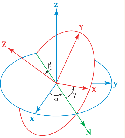

The \(XYZ\) system is fixed, while the \(xyz\) system rotates.

• Rotate the \(XYZ\) system about the \(z\) axis by \(\alpha\)
• Rotate the \(XYZ\) system about the now rotated \(X\) axis by \(\beta\)
• Rotate the \(XYZ\) system about the new \(Z\) axis by \(\gamma\)

A general rotation matrix can be written as the product of 3 \(M_{3\times 3}(\mathbb{R})\) matrices: \(A\mathbf{v}=A_3A_2A_1\mathbf{v}\). \[A=\pmatrix{ \cos\gamma&-\sin\gamma&0\\ \sin\gamma&\cos\gamma&0\\ 0&0&1 }\pmatrix{ 1&0&0\\ 0&\cos\beta&-\sin\beta\\ 0&\sin\beta&\cos\beta }\pmatrix{ \cos\alpha&-\sin\alpha&0\\ \sin\alpha&\cos\alpha&0\\ 0&0&1 }\] Note the operations are from right to left.

Arbitrary Basis for \(\mathbb{R}^n\)

An arbitrary basis is any set of vectors \(\{\mathbf{x}_1,\ldots,\mathbf{x}_r\}\) with \(\mathbf{x}_k\in\mathbb{R}^n\) such that if \[\sum^r_{k=1}\lambda_k\mathbf{x}_k=0\quad\textrm{then}\quad\lambda_1=\lambda_2=\ldots=\lambda_r=0\] for any other vector \(\mathbf{v}\) there exists \(v_i\in\mathbb{R}\) such that \[\mathbf{v}=\sum^r_{k=1}v_k\mathbf{x}_k\] Even if the number of elements is \(r=n\), they you may not have a basis. A set \(\{\mathbf{x}_1,\ldots,\mathbf{x}_n\}\) is a basis for \(\mathbb{R}^n\) if and only if \[\left(\begin{array}{c|c|c} &&\\ \mathbf{x}_1 & \cdots & \mathbf{x}_n\\ && \end{array}\right)\] is non degenerate.

Complex Vectors and Matrices

The norm

The length(norm) of a complex vector is defined using the complex conjugate: \[||\mathbf{v}||=\sqrt{\sum^n_{i=1}v^\star_iv_i}\] where we take the positive square root.

• To get the formula for \(||\mathbf{v}||\) we replace the transform operator with the dagger operator: \[||\mathbf{v}||^2=\mathbf{v}^\dagger\mathbf{v}\] where the \(\dagger\) operator represents the hermitian conjugate, given by \(\mathbf{v}^\dagger=\mathbf{v}^{\star T}\)

Given the complex matrix \(A\in M_{m\times n}(\mathbb{C})\), we have \[(A^\dagger)_{ij}=A^\star_{ji}\]

• We say that for a square matrix, it is hermitian if \(A^\dagger=A\).
• We say that for a square matrix, it is unitary if \(A^\dagger A=I\)

Scalar Product

The scalar product of two complex vectors \(\mathbf{u},\mathbf{v}\in\mathbb{C}^n\) is given by: \[\langle\mathbf{u},\mathbf{v}\rangle=\mathbf{u}^\dagger\mathbf{v}\in\mathbb{C}\]

Properties

• Skew symmetry \(\langle\mathbf{u},\mathbf{v}\rangle=\langle\mathbf{v},\mathbf{u}\rangle^\star\)
• (semi) Linearity \(\langle(\mathbf{u}+\mathbf{v}),\mathbf{w}\rangle=\langle\mathbf{u},\mathbf{w}\rangle+\langle\mathbf{v},\mathbf{w}\rangle\)
• \(\langle(\lambda\mathbf{u}),\mathbf{v}\rangle=\lambda^\star\langle\mathbf{u},\mathbf{v}\rangle\) and \(\langle\mathbf{u},(\lambda\mathbf{v})\rangle=\lambda\langle\mathbf{u},\mathbf{v}\rangle\)

The natural basis \(\{\mathbf{e}_1,\ldots,\mathbf{e}_n\}\) remains an orthonormal basis for \(\mathbb{C}^n\). I.e. \(\langle\mathbf{e}_i,\mathbf{e}_j\rangle=\delta_{ij}\) .\[\mathbf{v}=\sum^n_{i=1}v_i\mathbf{e}_i\quad\textrm{and}\quad v_i=\langle\mathbf{e}_i,\mathbf{v}\rangle\] but note, in general: \(v_i\neq\langle\mathbf{v},\mathbf{e}_i\rangle\)

Eigenvalues and Eigenvectors

Given a square matrix \(A\in M_{n\times n}(\mathbb{C})\), the complex number \(\lambda\) is an eigenvalue of \(A\) with the corresponding eigenvalue \(\mathbf{v}\in\mathbb{C}^n,\;\mathbf{v}\neq\mathbf{0}\) if it satisfies \[A\mathbf{v}=\lambda\mathbf{v}\]

Observe that if \(\mathbf{v}\) is an eigenvector then so is \(\mu\mathbf{v}\) for all \(\mu\neq 0\). We consider \(\mathbf{v}\) and \(\mu\mathbf{v}\) representing the same eigenvector.

Also note that \[\mathbf{0}=A\mathbf{v}-\lambda\mathbf{v}=(A-\lambda I)\mathbf{v}\] Since \(\mathbf{v}\) cannot equal \(\mathbf{0}\), the inverse of \((A-\lambda I)\) cannot exist, meaning that it is degenerate. Hence \[\boxed{\det(A-\lambda I)=0}\] Let \(p_A:\mathbb{R}\to\mathbb{R}\) be the polynomial \[p_A(\lambda)=(-1)^n\det(A-\lambda I)\] which is called the characteristic polynomial. We can set this to zero and solve for \(\lambda\) which will be an eigenvalue of \(A\). We can then use each eigenvalue \(\lambda_i\) to find the corresponding eigenvector using the homogeneous linear equation: \[(A-\lambda_iI)\mathbf{v}_i=\mathbf{0}\]

Diagonalisation of Matrices

A (square) matrix \(A\in M_{n\times n}(\mathbb{C})\) is diagonalisable if there exists an invertible matrix \(B\in M_{n\times n}(\mathbb{C})\) and a diagonal matrix \(\Lambda\) such that \[A=B\Lambda B^{-1}\] Let \(B\in M_{n\times n}(\mathbb{C})\) be the matrix constructed from the eigenvectors of \(\mathbf{v}_1,\ldots,\mathbf{v}_n\) of \(A\), and let \(\Lambda\) be constructed from the eigenvalues: \[B=\left(\begin{array}{c|c|c} &&\\ \mathbf{v}_1 & \ldots & \mathbf{v}_n\\ &&\\ \end{array}\right) \quad\textrm{and}\quad \Lambda=\pmatrix{ \lambda_1 & & 0\\ & \ddots &\\ 0 & &\lambda_n }\]

Some Properties

• The determinant of a matrix is the product of all its eigenvalues with multiplicity. (Repeats are included). (Even if the matrix is not diagonalisable). \[\det(A)=\prod_i\lambda_i\]
• The trance of a matrix is the sum of all of its eigenvalues with multiplicity. (Even if the matrix is not diagonalisable). \[\textrm{Tr}(A)=\sum_i\lambda_i\]
• There is no relationship between whether a matrix can be diagonalised and whether it is invertible.
• If all of the eigenvalues of the matrix are distinct (i.e. have multiplicity 1), then the matrix \(A\) is diagonalisable.
• Symmetric (\(A^T=A\)) can all be diagonalised.
• Hermitian (\(A^\dagger=A\)) can all be diagonalised.
• Orthogonal (\(A^TA=I\)) can all be diagonalised.
• Unitary (\(A^\dagger A=I\)) can all be diagonalised.

Mutually Diagonalising Two Matrices

Given two matrices \(A,C\in M_{n\times n}(\mathbb{C})\) is it possible to mutually diagonalise these matrices? E.g. \[A=B\Lambda B^{-1}\quad \textrm{and}\quad C=B\Gamma B^{-1}\] We can do this if both \(A\) and \(C\) are each diagonalisable and they commute: \[[A,C]=AC-CA=0\]In quantum mechanics if \(A\) and \(B\) commute, and are therefore mutually diagonalisable Hermitian matrices, then they represent physical quantities which can be “known” at the same time. I.e. measuring \(A\) and then \(B\) we get the same result as if we measured \(B\) and then \(A\).

Systems of Linear Equation

Let a system of \(m\) linear equations with \(n\) unknowns. \[\begin{array}{c c c c} A_{11}x_1+&\ldots&+A_{1n}x_n&=b_1\\ \vdots & \vdots & \vdots & \vdots\\ A_{m1}x_1+&\ldots&+A_{mn}x_n&=b_m \end{array}\] or in matrix form \[A\mathbf{x}=\mathbf{b}\quad\implies\quad \pmatrix{ A_{11} & \ldots & A_{1n}\\ \vdots & \ddots & \vdots\\ A_{m1} & \ldots & A_{mn} }\pmatrix{ x_1\\ \vdots\\ x_n }=\pmatrix{ b_1\\ \vdots\\ b_m }\]

Solving when \(m=n\)

If \(A\) is non degenerate, \((\det(A)\neq 0)\), then \(A^{-1}\) exists, in which we can multiply both sides of the equation by it to solve for \(\mathbf{x}\) If \(\det(A)=0\), there are either many, or no solutions.

Homogeneous Linear Systems

Given the linear system \(A\mathbf{x}=\mathbf{0}\), where \(A\in M_{m\times n}\mathbb(R)\) this is a homogeneous linear system of equations. The solution set is \[S=\{\mathbf{x}\in\mathbb{R}^n|A\mathbf{x}=\mathbf{0}_m\}\]

• The zero vector \(\mathbf{0}_n\) is always a solution: \(\mathbf{0}_n=\mathbf{0}_m\), and \(\mathbf{0}_n\in S\).
• We can add solutions to produce a new solution.
• We can multiply a solution by a scalar to produce a new solution.

Hence we can present \(S\) as \[S=\left\{\lambda_1\mathbf{v}_1+\ldots+\lambda_r\mathbf{v}_r|\lambda_1,\ldots,\lambda_r\in\mathbb{R}\right\}\] for some vectors \(\mathbf{v}_1,\ldots\mathbf{v}_r\in\mathbb{R}^n\).

Inhomogeneous Linear Systems

Given the linear system \(A\mathbf{x}=\mathbf{b}\), where \(\mathbf{b}\neq\mathbf{0}\), this is a inhomogeneous linear system of equations. The solution set is \[S=\{\mathbf{x}\in\mathbb{R}^n|A\mathbf{x}=\mathbf{b}\}\]

• The system may be inconsistent, and there may be no solutions: \(S=\emptyset\).
• The linear system has a homogenous part \(A\mathbf{x}=\mathbf{0}\).
• If \(z\) is a solution to the inhom. equation, and \(v\) is a solution to the hom. equation \(v+z\) is also a solution to the inhom equation.

Hence we can present \(S\) as \[S=\left\{\lambda_1\mathbf{v}_1+\ldots+\lambda_r\mathbf{v}_r+\mathbf{z}|\lambda_1,\ldots,\lambda_r\in\mathbb{R}\right\}\] i.e. we need all of the solutions to the homogeneous equation and only one solution to the inhomogeneous equation.

Ordinary Differential Equations

Given a function \(x(t)\), and its derivatives \(\dot{x}\;\textrm{and}\;\ddot{x}\).

• And ODE is an equation which contains at least one ordinary derivative as seen above.
• We can have systems of equations, i.e. \[\left\{\;\;\begin{align}&\ddot{y}+(\dot{x})^4+e^y=7\\&\ddot{x}+\sin(\dot{y})+e^y=0\end{align}\right.\]
• We need to find solutions \(x(t),\;y(t)\) that when substituted into the equations above, holds.
• In general this is very hard or impossible.

Linear ODEs

All linear homogeneous ODEs or system of ODEs can be written in the form \[\frac{d}{dt}\mathbf{x}(t)=A(t)\mathbf{x}(t)\] All linear inhomogeneous ODEs or system of ODEs can be written in the form \[\frac{d}{dt}\mathbf{x}(t)-A(t)\mathbf{x}(t)=\mathbf{b}(t)\] where \(\mathbf{b}(t)\) does not contain any dependent variable.

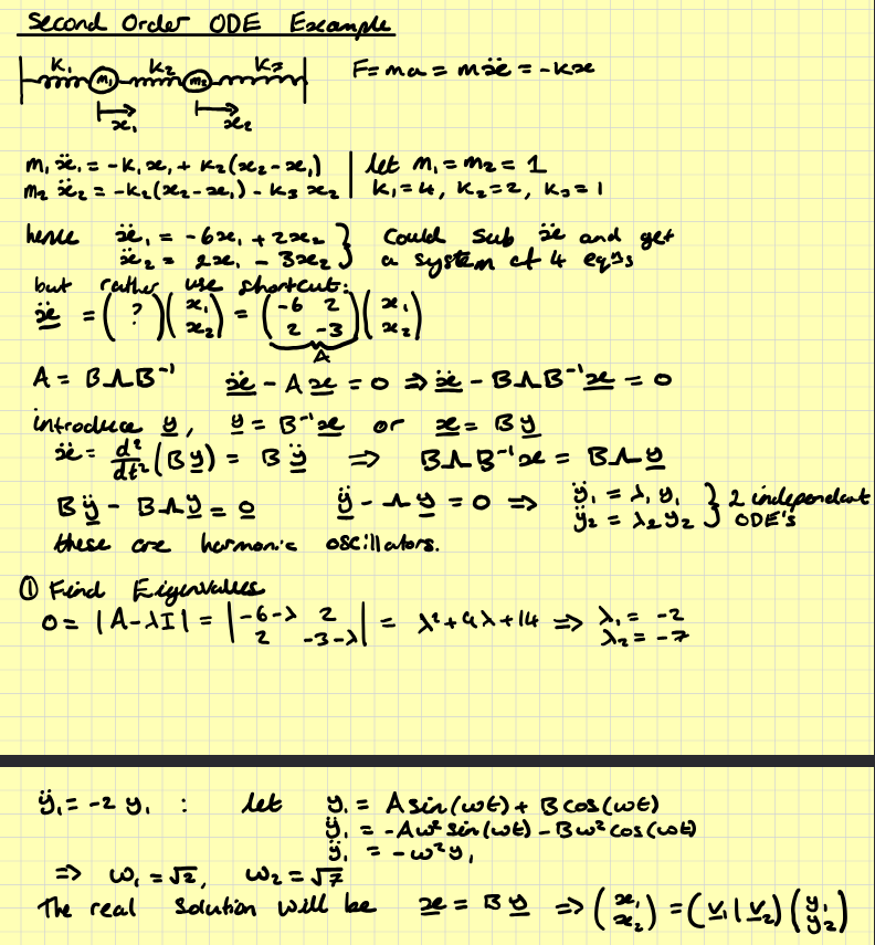
What happens when one of the equations contains higher derivatives, second order or above?We simply introduce a new dependent variable!I.e. \(x_1(t)=x(t)\), and \(x_2(t)=dx/dt=dx_1/dt\)

Example

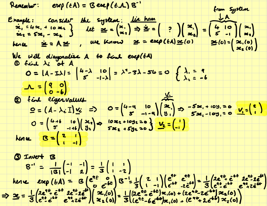
If we have a matrix ODE \[\frac{d\mathbf{x}}{dt}=A\mathbf{x}(t)\] where \(A\) is a constant matrix (not dependent of \(t\)), we say we have a linear homogeneous ODE with constant coefficients. We can always solve linear ODEs with constant coefficients. The solution is given by \[\mathbf{x}(t)=\exp(tA)\mathbf{x}(0)\] where we can use \[\exp(tA)=\sum_{r=0}^\infty\frac{t^rA^r}{r!}\]

There is no formula for \(\frac{d\mathbf{x}}{dt}=A(t)\mathbf{x}\)

To calculate \(\exp(tA)\) we diagonalise \(A\). Set \(A=B\Lambda B^{-1}\) then \[\exp(tA)=B\exp(t\Lambda)B^{-1}\] (since \(A^r=B\Lambda^rB^{-1}\)) This is simple as the diagonal matrix only contains entries on the diagonals, such that \[\exp(tA)=\pmatrix{e^{t\lambda_1} & & 0\\& \ddots &\\0 & & e^{t\lambda_n}}\]

Example

Proving with method of induction

• We prove the statement \[A^r=B\Lambda^rB^{-1}\] using method of induction.
• This method consists of two steps: 1. prove the statement for a particular value of \(r\). 2. prove the statement works for \(r=p+1\).

System of Linear Inhomogeneous ODEs

• The matrix ODE of the form \[\frac{d\mathbf{x}}{dt}=A\mathbf{x}(t)+\mathbf{b}\] where \(A\) is a constant matrix and \(b\) is a constant vector is called a system of linear inhomogeneous ODE with constant coefficients.
• Given a solution \(y(t)\) to a linear inhomogeneous ODE and \(x(t)\) is a solution to the homogeneous part, then \(z(t) = x(t) + y(t)\) is also a solution to the linear inhomogeneous equation
• \(y(t)\) can be any particular solution, whatever is easy to find
• Using it and the solution \(x(t)\) of the homogeneous part we obtain the general solution of the linear inhomogeneous ODEs

Example

Part III - Dirac \(\delta\) Function

The Dirac delta function is written \(\delta(x)\), where \(x\in\mathbb{R}\).

• Actually, it is not a function. This type of objects is called generalized function.
• Regular function relates each number \(x\in\mathbb{R}\) to a number \(y\in\mathbb{R}: y=f(x)\);
• Generalized function relates each regular function \(f\) to a number \(y\in\mathbb{R}\)
• Given any (continuous) function \(f\) we define the generalized function \(\delta(x)\) as: \[\int^\infty_\infty f(x)\delta(x)dx=f(0)\]
• From above it follows that \[\int^\infty_\infty\delta(x)dx=1\]
• Generalized function \(\lim_{x\to0}\delta(x)=0\), however \(\delta(0)=+\infty\). This is why it is a generalized function.
• \(\delta(ax)=\delta(x)/|a|\)
• \(\int^t_\infty\delta(x)dx=H(t)\implies H'(t)=\delta(t)\)